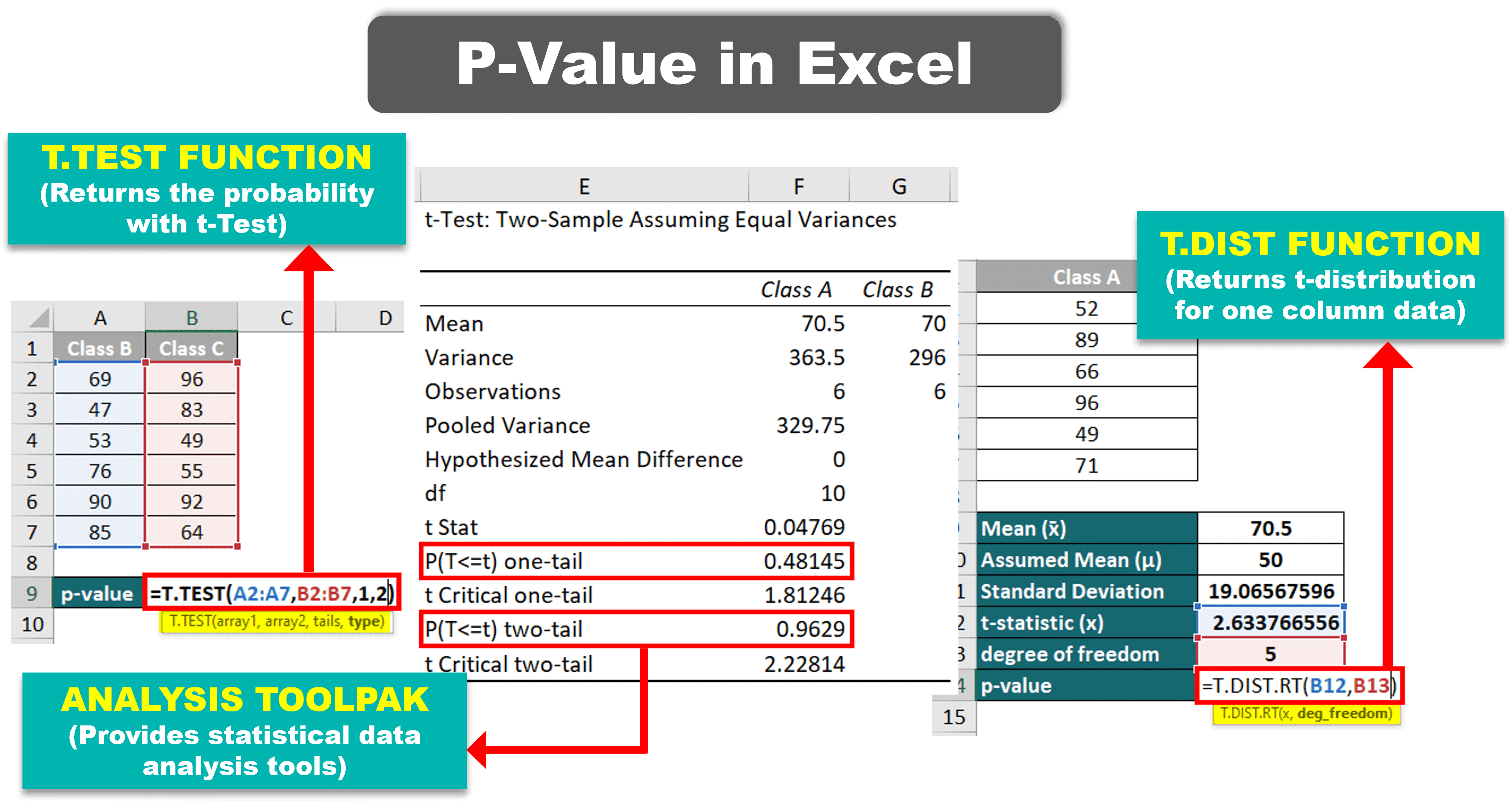
Let’s get our hands dirty. Open Excel, put your two groups in columns A and B. In a random cell, type this: =T.TEST(A1:A100, B1:B100, 2, 2). That 2,2 means two-tailed and equal variance—the everyday toolkit of data analysis.
Hit Enter, and you’ll get a number between 0 and 1. That’s your P-value. If it’s below 0.05, you’ve got a statistically significant result. If it’s above? Don’t panic—it just means your data is shouting into the void, and that’s okay.
Pro tip: If you get a number like 0.000023? That means Excel is basically crying with joy. Your finding is about as likely as a cat successfully using a toilet—technically possible, but incredibly rare.
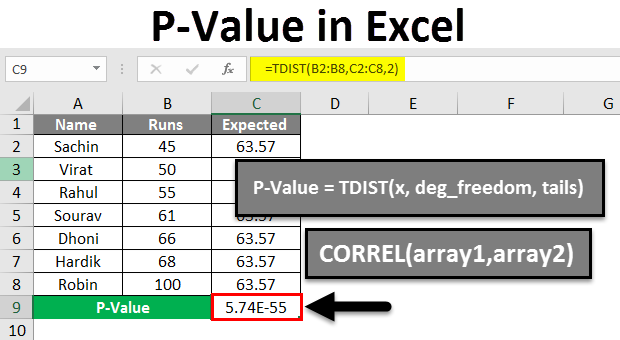 P-Value in Excel | How to Calculate P-Value in Excel?